IO:I

After being offline since 2020 following issues with its cryostat, IO:I was officially decommissioned in 2023 to be replaced with LIRIC. The IO:I information presented here is for historical purposes only.

Introduction

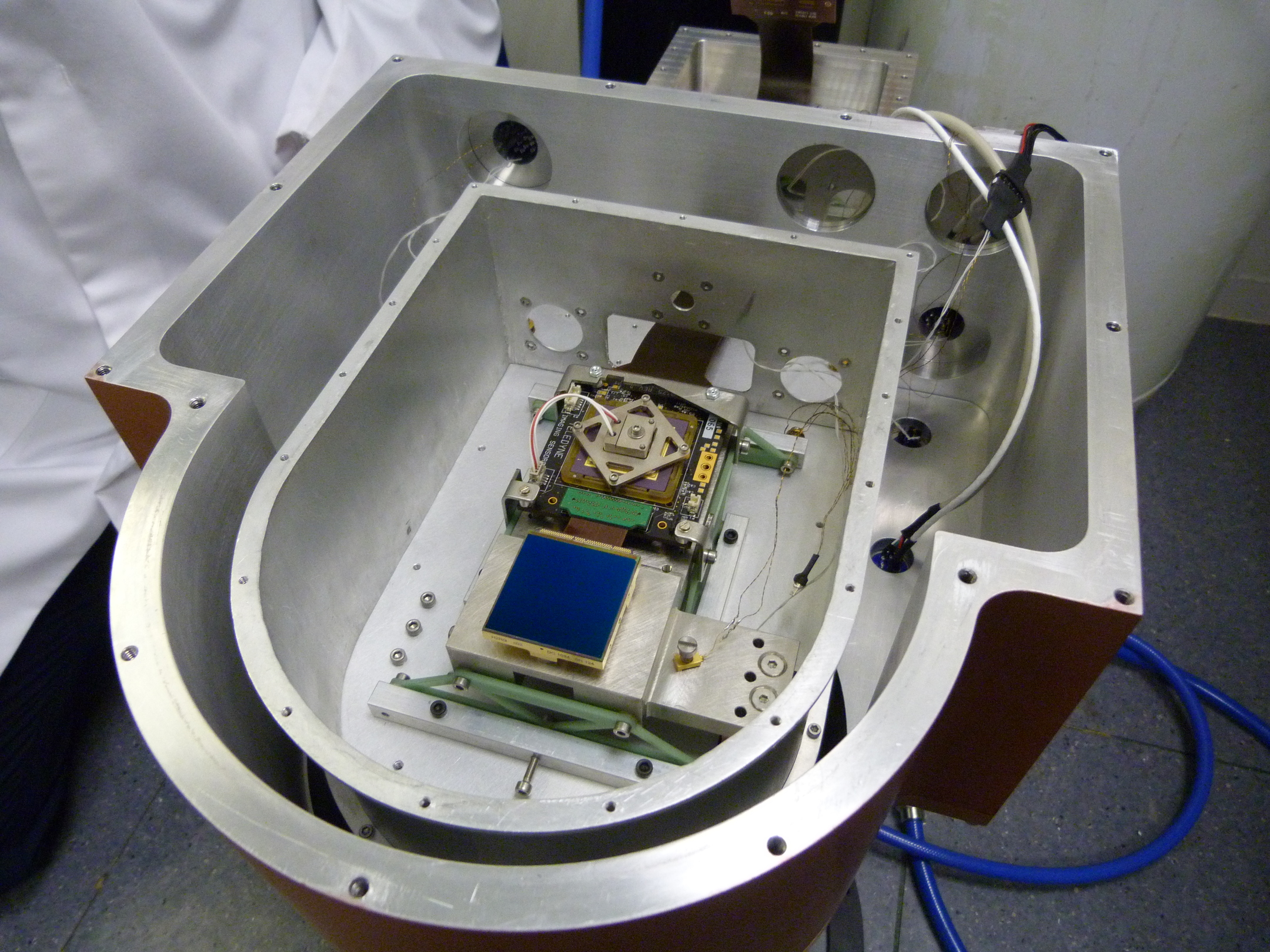
IO:I is the near-infrared imaging component of the IO suite of instruments. It uses a 2048x2048 pixel Hawaii 2RG 1.7μm cutoff detector with a field of view of 6.3 arcminutes, a pixel scale of 0.18 arcsec, and currently a single H-band (1.5-1.8 micron) filter. It became available as a common-user instrument in August 2015.

The instrument design is described in greater detail in R.M. Barnsley, H.E. Jermak, I.A. Steele, R.J. Smith, S.D. Bates, C.J. Mottram, "IO:I, a near-infrared camera for the Liverpool Telescope", J. Astron. Telesc. Instrum. Syst. 2(1), 015002 (Mar 04, 2016). (http://dx.doi.org/10.1117/1.JATIS.2.1.015002).

Contents

• Specification
• Filters
• Integration Time
• Sensitivity and Sky Brightness
• Bright stars and defocus
• Dither Patterns
• Autoguiding
• Overheads
• Total Observing Time Calculation
• RTML and Automated Followup
• Dates of Hardware Changes
• Data Reduction Pipeline
  • Data Processing Details
  • Filenames and FITS Extensions

Specification

Detector	Teledyne 2048 x 2048 Hawaii-2RG 1.7μm cutoff HgCdTe Array
Pixel size	18.0 x 18.0 microns
Pixel scale	0.184 arcsec/pixel (unbinned)
Field of view	6.27 x 6.27 arcmin
Preamp gain	18dB
Read noise (2-pair Fowler mode)	15e-
Dark current	<0.01e-/s
Binning	None initially available
Min./Max. Exposure	from 1×6sec to 34×60=2040sec
Readout time	1.45s (non-destructive)
Windowed modes	None initially available
Gain	1.5e-/ADU
Saturation Limit	93ke-
Filter Set	H only [Transmission data]
Quantum Efficiency (figures supplied by manufacturer)	Wavelength (nm) Quantum Efficiency (%) 800 58 1000 57 1230 73 1500 86 1720 50

Filters

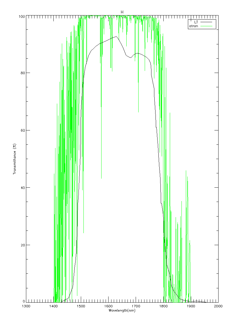
At present, the IO:I cryostat accommodates a fixed H filter, meaning the red cutoff is defined by the detector, not the filter.

Alternative configurations exist with either a fixed J filter or a split-field J+H filter in which half of the array sees the J-band, the other the H-band; the effective field-of-view is halved but targets may be observed near-simultaneously in both bands by nodding them between the two filter halves. If you have a requirement for either of these J-band configurations please contact us. For the current semester we are committed to offering H only but configuration in future semesters will be based on demand from applicants.

A transmission plot for the H filter is displayed at right (click for bigger version). A model atmospheric window (ATRAN) has been overplotted. The filter transmission data as measured on the bench and transformed to predicted performance at operating temperature are available as text files.

Integration Time

IO:I is always used with a sequence of short, dithered exposures that are coadded by the pipeline. Minimum exposure time is defined by the hardware read time overheads. The maximum is limited by the background count rate and depends on the currently installed filter.

• The minimum exposure per frame is 6 sec.
• The maximum recommended exposure in H-band is 60 sec.

Due to memory limitations in the IO:I control computer, the number of dithered exposures that can be made in each multrun is currently limited to 34 frames, giving the deepest possible single multrun integration of 34×60 = 2040sec.

Sensitivity and Sky Brightness

Signal to Noise estimates for IO:I are available from the Imaging Exposure Time Calculator. Measured sky brightness pre-realuminisation (before July 2015) is 12.5 mag/sq arcsec.

As an example, an exposure time of 10s will allow observations of 14th magnitude targets with a SNR of ~100 for a single dither. Increasing the number of dithers yields an increase in the SNR at a factor proportional to the square of the number of dithers. Increasing the number of dithers also has the advantage of improving the quality of the sky subtraction.

The exposure time and number of dithers should be selected such that good sky subtraction can be achieved without sky saturation.

Bright stars and defocus

Either positive or negative offsets are allowed in the phase2ui, but defocus greater than 0.3mm in either direction is not recommended. Such strong defocus will lead to failure of the dither cross-matching algorithm making it impossible for the automated software pipeline to produce any reduced data products for you.

The diameter a star will appear on the detector is very simply calculated from the optical prescription of the telescope and detector pixel scale. For defocus (DF) expressed in mm, the diameter of the defocused star in the image will be 60.5 * DF pixels.

Of more importance is the decrease in peak brightness as a function of defocus. Here it is only possible to offer a general rule-of-thumb since it will be dependent on external factors such as the atmospheric seeing. Defocus of 0.3mm will yield a peak counts of approximately 35% of a focused image. A peak counts of 50% is achieved with roughly 0.2mm and 80% by defocus of 0.1mm. Defocus greater than 0.3mm is not recommended.

Dither Patterns

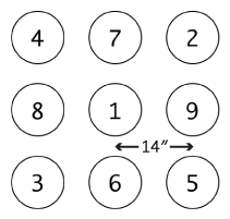
The dither pattern is hard-coded to cycle through a 3x3 grid of 9 positions, repeating up to a maximum of 34 exposures (almost four 9-frame cycles). Any number up to 34 can be made - the cycle can be interrupted at any time - so you are not restricted to multiples of 9 exposures. Equally, if you need deeper integrations then multiple runs may be requested, each up to 34 frames long.

	Click to start animation.
The 3x3 grid dither pattern is spaced 14 arcseconds apart in RA and DEC, and the nine frames are exposed in this numerical order.	Animation showing how an example 14-dither IO:I image is built up. Dithers cycle through and then partly repeat the 3x3 grid to make the final image. Dither offsets exaggerated for clarity. Click picture to start animation; click elsewhere to stop.	Dither offset to scale: 14 arcseconds imposed on a 6.27 arcminute frame. A narrow frame around the edge of the image may therefore have a smaller total integration time in the final stack.

As stated above, you are not restricted to 9 dithers, you need only do 5 to obtain a decent result. But if you want more, you are free to do so, up to 34. Below is a selection of example different patterns and the advantages and disadvantages of each. Again, the dither offsets in the diagrams are exaggerated for clarity.

No. of dithers	Details
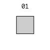	A single pointing. Though technically possible this is strongly discouraged. The automated reduction pipeline will not be run because it is dependent on the dither for sky subtraction, so only the raw data will be available to you.
	This is sufficient to do a simple sky subtraction for point sources, but is not ideal for deriving the best flat fields.
	Gives a "cross"-shaped mosaic of five pointings. It is the best choice for general purpose use, allowing good sky subtraction and flat field generation.
	Gives a 3x3 "square" mosaic of nine or more pointings. It allows the generation of the best quality flat fields, and is recommended for crowded or complex fields.

Autoguiding

All IO:I observations should be acquired with the autoguider set to "Off". This is to allow the telescope to dither between exposures. With the short exposures required for near-IR imaging, observing without the auto-guider locked should not seriously impact the image quality obtained. The automated data reduction pipeline will align and stack all the individual frames for you.

Overheads

IO:I data is taken with 2-pair Fowler sampling. This means that 2 frames are taken at the start of the exposure (pedestal frames 1&2), and two at the end (readout frames 3&4). A single readout time separates the frames in both the pedestal and readout pairs. As per the standard prescription for Fowler sampling, the average of the differences between frames 1&3 and 2&4 is taken for each sequence. These pairs have equivalent exposure times.

Because the array has no shutter, the true exposure time requested by the user via the Phase2UI interface is amended automatically by the robotic software to account for the readout time overhead; this is necessary to obtain the exposure time that the user has requested. The amendment is opaque to the user. As the array is read non-destructively, readout overheads are mostly absorbed into the requested exposure length itself and have little impact alongside the other overheads.

Each dither in the sequence therefore incurs an overhead of:

• application of offset for each dither: 5s
• processing time for each dither: 10s

Total Observing Time Calculation

The total telescope time used (T_total) will be a combination of:

• acquisition time (slew to target): T_acq = 60s
• application of offset for each dither: T_off = 5s
• exposure time for each dither: T_exp
• processing time for each dither: T_proc = 10s

such that for a pattern of N dithers:

T_total = T_acq + N*(T_off + T_exp + T_proc).

Example: a 9-pattern dither of 30s per exposure (N = 9, T_exp = 30s):

T_total = 60 + 9*(5 + 30 + 10) = 465 seconds

RTML and Automated Followup

IO:I can accept observation requests formated in Remote Telescope Markup Language (RTML) which allows you to automatically trigger certain observations from within your own autonomous software. We provide a command line based utility which can format RTML packets for you, making it easy to integrate observing requests into a shell script or other data processing pipeline. For some use cases it might also be easier for users to upload all their observing requests from the command line instead of using the phase2ui. The facility is available to all users who have TAG-awarded time allocations. Please contact us if this sounds of interest and we can provide full user instructions.

Dates of Hardware Changes

For the benefit of observers performing long term monitoring we here summarize the dates of major hardware changes that could potentially lead to changes in photometric calibrations.

Vignetted frame corner (November 2015 – 15th August 2016):
There is an intermittent artifact in the lower-right corner of the frame, caused by imperfectly-corrected vignetting. The maximum photometric error is typically 0.1 mag, and 0.2 mag maximum for the worst case. Sources more than 300 pixels from the frame corner are completely unaffected. The small image to the left (Click image to enlarge) shows the affected area, grey-scaled to greatly exaggerate the visual appearance of the effect. A hardware fix was installed 2016-08-15 and the dark patch does not appear after that date.

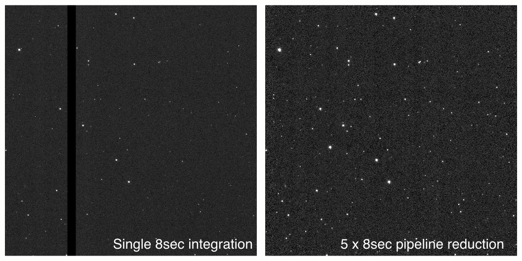
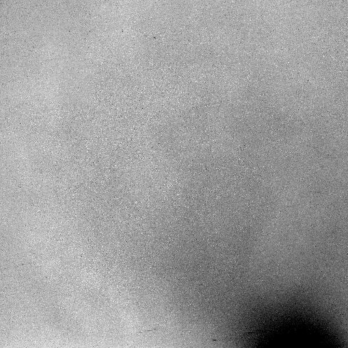
Intermittent dead columns in array read-out:
From 22nd March 2017 a fault developed in a single array read channel. This led to a completely blank image section with a width 1/32nd of the full array area. Since IO:I observations are generally always obtained with offset dithers, the automated reduction pipeline is able to reject the failed pixels and construct a clean final image. There is no known impact on the accuracy of photometry though the effective signal-to-noise could of course be reduced in the image strip being constructed from fewer dithers. The example image to the left shows both a single 8sec integration and the pipeline generated stack from a typical dithered sequence of five 8sec exposures. (Click image to enlarge.) The problem is intermittent.

• 2017-03-22 – 2017-10-22: Single dead read channel.
• 2017-10-22 – 2017-11-07: Two dead read channels. Stacks generated from at least five dithers are still OK.
• 2017-11-07 – 2018-10-25: No problem. Complete array images.
• 2018-10-25 – Ongoing : Single dead read channel.

Array temperature:
From commissioning until 7th November 2017 the IO:I array was operating in the range 78–83K. From 8th November 2017 onwards the array is operating slightly warmer at approximately 100K. Direct comparisons of photometric standards obtained at 80K and 100K have so far revealed no measurable difference.

2018-06-27 Tertiary feed mirror cleaning gave a significant step-change increase in total throughput.

Data Reduction Pipeline

The pipeline software are described in greater detail in IO:I, a near-infrared camera for the Liverpool Telescope, R.M. Barnsley et al, 2016, J. Astron. Telesc. Instrum. Syst, Vol. 2 ( http://dx.doi.org/10.1117/1.JATIS.2.1.015002). A brief overview is provided here.

Reductions are applied to IO:I images before the data are passed to users. This includes bias subtraction, CDS, nonlinearity correction, flat fielding, bad pixel masking, sky subtraction and frame registration/stacking (if possible). A library of the current calibration frames is maintained as part of the data archive and updated daily so that images are always reduced using the latest available calibrations.

The pipeline software depends on the pointing dither to perform sky subtraction which means undithered, single frame, snap-shot observations will not be processed and will be distributed to the observer completely raw.

Each of the operations performed by the pipeline are described below.

• Bias Subtraction

  
  

  The H2RG array comes with 8 columns and 8 rows of reference pixels. These pixels are not connected to a photodiode but are read out in the same way as active pixels, allowing the reference level to be subtracted off.

• CDS

  
  

  Fowler pairs are made and averaged to reduce the read noise. This yields a single frame per dither position.

• Nonlinearity Correction

  
  

  Nonlinearity corrections are performed on a per pixel basis, correcting for the nonlinear architecture of the pixel unit-cell. After correction, residual linearity is expected to be no greater than 1%.

• Flat Fielding

  
  

  Twilight flats are automatically obtained and averaged to produce a library flat.

• Bad Pixel Mask

  
  

  Due to the greater number of defective pixels in IR arrays, a bad pixel mask is applied to mask those pixels with <35% QE and/or >1% residual nonlinearity.

• Sky Subtraction

  
  

  A median sky is built from the CDS frames at each dither position. This sky is then scaled to match the science frame and subtracted. Note that if the source being observed is extended and an offset sky taken, then pipelined products with _SS extension names should be disregarded and the user is encouraged to perform their own sky subtraction.

• Frame Registration/Stacking

  
  

  If enough sources are present in the field observed, the pipeline will attempt to register the CDS images from all dither positions and stack (co-add) them.

Data Format: Filenames and FITS Extensions

For an observation sequence of N dithers, normally N+1 processed output files will be made available to the user. Filenames follow the usual LT conventions and are in the form "i_e_20150523_1_X_0_R.fits", where X represents the dither frame number from 1 – N, and R is a status flag that defines what level of processing has been applied.

Reduction Flag R	Details
1	Reduced single dither image. X is set to the frame number in the dither sequence 1 – N. The FITS contains two images. The primary image (EXTNAME="IM_SS") has been sky-subtracted and the first image extension (EXTNAME="IM_NONSS") is a non-sky-subtracted version. Other than sky subtraction, the two images are processed identically.
2	Aligned and co-added stack of the full sequence of N frames. X in filename is set to 0. If the pipeline was unable to align and stack the N dithers this *_2.fits file will not be created.
0	Raw data as read from the detector array. For an N dither position observation there are 4N FITS files. For each exposure the four FITS files are the four separate correlated double sampling reads of the detector array arranged as two Fowler pairs, two reference reads before the integration and two data reads after the integration. The raw data are generally not distributed to observers because the automated pipeline which performs the CDS combination is reliable, but they are available if needed.

Extraction using the Starlink software

Starlink users may extract the appropriate extension using the CONVERT:FITS2NDF command, appending the filename with the extension they wish to extract in brackets. The result is a single extension .SDF file.

For example, to extract the stack, sky-subtracted image from the multipart FITS file i_e_20150523_1_0_0_1.fits use:

 
  > convert 
  > fits2ndf "i_e_20150523_1_0_0_1.fits[0]"
  

Or alternatively, you can access the required HDU by using the corresponding EXTNAME key:

 
  > fits2ndf "i_e_20150523_1_0_0_1.fits[SK_SS]"
  

Extraction using DS9

DS9 users may view the available extensions by adding -multiframe on the terminal command line:

 
  > ds9 -multiframe i_e_20150523_1_0_0_1.fits
  

A frame extraction can be achieved by adding the -frame and -savetofits parameters, specifying the frame to be extracted (frame 1 corresponds to the primary HDU):

 
  > ds9 -multiframe i_e_20150523_1_0_0_1.fits -frame 1 -savefits output.fits -quit