MOPTOP on workbench with its top removed. Image © 2022 Iain Steele.
MOPTOP
- Introduction
- Current Status
- Description
- Technical Spec
- Operational Principle
- Exposure Time
- Brightest Targets and Saturation
- Filename Convention
- Data Reduction Pipeline
- Deriving Polarisation
Introduction
MOPTOP, the Multicolour OPTimised Optical Polarimeter, is specially designed for time domain astrophysics. It takes the already-novel aspects from the RINGO series of polarimeters and add a unique optical dual-camera configuration to both minimize systematic errors and provide the highest possible sensitivity.
MOPTOP's design enables the measurement of polarisation and photometric variability on timescales as short as a few seconds. Overall the instrument allows accurate measurements of the intra-nightly variability of the polarisation of sources such as gamma-ray bursts and blazars, allowing the constraint of magnetic field models to reveal more information about the formation, ejection and collimation of jets.
MOPTOP was mounted on the telescope for commissioning and calibration in early 2020, just before coronavirus lockdown travel restrictions between the UK and the Canary Islands came into force. The instrument began observing robotically in October 2020.
Current Status
ONLINE
Description
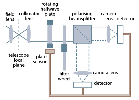
MOPTOP is a dual-beam polarimeter. Incoming collimated light first passes through a continuously rotating half-wave plate which modulates the beam's polarisation angle. The polarised light then passes through a wire-grid polarising beamsplitter. This splits the light into the p and s polarised states and sends the now-separate beams through filter wheels to a pair of low-noise fast-readout imaging cameras.
Image acquisition is electronically synchronised to the rotation angle of the half-wave plate. This combination of half-wave plate and beamsplitter provides about twice as much throughput as conventional polarimeters that use polaroid filters as the analyser.
Technical Spec
| Optical Performance |

|
|---|---|
| Cameras |
Current cameras (20th March 2022 – present):
|
Previous cameras (10th October 2020 – 19th March 2022):
|
|
| Half-wave Plate |
|
| Beamsplitter |
|
| Filters |
|
IMPORTANT - Epochs of hardware and software changes
MOPTOP's cameras and imaging modes have changed several times over the years. The relative physical alignment between optical components is critical to data reduction, so it is important to ensure that standards, stokes parameters, and science data, are all from the the same "hardware epoch" defined by these dates of hardware/software changes.
Dates of hardware and imaging mode changes
- 2020-10-01 — Instrument commissioning begins, using two Andor Zyla cameras
- 2021-03-09 — Andor camera 1 replaced with same model after previous camera 1 fault
- 2021-09-20 — Switch to imaging only with Andor camera 1, after fault with Andor camera 2
- 2022-03-20 — Both Andor cameras replaced with PCO cameras, imaging with two cameras again
- 2024-09-13 — Primary mirror realuminised
Please feel free to contact the LT Support Astronomer to discuss the impact any of these changes might have had on your data.
Operational Principle
Key to MOPTOP's operational principle is the use of a half-wave plate to modulate the polarisation angle of the incoming beam, plus camera systems that can simultaneously record the resulting two orthogonal polarization states. A 22.5° rotation of the waveplate rotates the polarization angle of the beam by 45° effectively swapping the q and u Stokes parameters. This allows variations in the polarisation response of MOPTOP to be corrected by a differential technique, reducing systematic errors to a level below those produced by RINGO3.
Sixteen images are acquired in each camera for every rotation of the waveplate. As four frames in succession are needed to make one polarisation measurement, four measurements are therefore obtained per complete rotation.
The figure below left shows exposure times and angles for each rotation position. The blue shaded areas in the top figure indicate the waveplate angle for each exposure. The white areas denote the readout time. The plot below right shows waveplate angle, and the resulting electric vector position angle (EVPA), as a function of time.
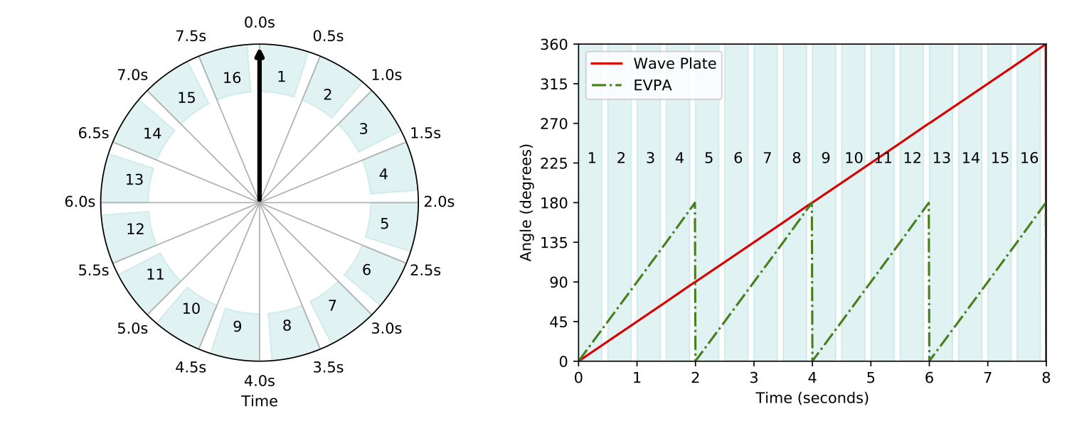
Left: MOPTOP operational principle, showing the sequence of frames taken at different angles of the rotating wave plate as a function of time when operating in "fast mode" (one revolution in 8 sec — more info on modes below). Exposure of a frame simultaneously begins on both cameras 0.5s after the previous one, with the waveplate rotation angle having increased by a total of 22.5° over that time period. The blue shaded areas indicate the time the shutter is open (duration 0.4s), with the shorter white regions indicating the 0.1s readout gaps between frames. Frames are numbered 1-16. Right: waveplate rotation angle and resulting EVPA rotation of the incoming beam as a function of time. (from Shrestha et al. (2020))
"Fast" and "Slow" Speed Modes
| attribute | speed mode | |
|---|---|---|
| fast | slow | |
| rotation period (s) | 8 | 80 |
| frame interval (s) | 0.5 | 5.0 |
| frame exposure time (s) |
0.4 | 4.0 |
The half-wave plate can rotate at two different speeds, chosen by the observer. In "fast mode", the waveplate completes one revolution in 8 seconds (7.5rpm), while in "slow mode" one revolution lasts 80 seconds (0.75rpm).
In fast mode, each of the 16 rotation positions is imaged every 0.5 seconds. Exposure time is actually 0.4s, with 0.1s allowed for readout time. In slow mode, positions are imaged every 5.0s with exposures lasting 4.0s. The extra second until the next exposure is both for readout and to ensure the same angle is swept out by the rotator per exposure in slow as well as fast mode, so that we can interchange standards in both modes.
Observers should choose fast mode if the target is brighter than mv = 12 (See Brightest Targets and Saturation), or if there is a need for time resolution better than a few seconds in polarisation measurement. Using slow mode whenever possible is recommended, as this yields a smaller data set which is easier to handle.
Cassegrain Rotator
We also strongly recommend that all the observations are made with the cassegrain mount angle set to zero degrees.
Exposure Time
MOPTOP exposure times are treated differently compared to the other instruments. Each rotation produces 16 exposures, and MOPTOP only observes for a complete number of rotations. Therefore as the time you enter into the Phase2UI corresponds to the number of rotations rather than individual exposures, we refer to this time as the "duration" to distinguish it from the individual exposures.
A complicating factor however is that MOPTOP rounds down the duration to correspond to a complete number of rotations. So if a duration of 200s in slow mode (period 80s) is entered, then only two rotations (2×80=160s) would be observed, because three rotations (240s) would go over the duration time.
If however 200s was absolutely necessary, then three rotations would have to be used. You should therefore enter the duration for the integer number of rotations that cover the integration time you want.
Another consideration is that the individual exposure times are not simply the rotation period divided by 16 (i.e. 0.5s or 5.0s). Frame readout takes up 0.05s per exposure, so the actual exposure times are 4.95s or 0.45s for slow and fast modes respectively. This difference can add up over time for long durations, and if total integration time on sky is important to the observation then this extra effect must be taken into account.
An equation to calculate the duration td to enter into the Phase2UI to make sure a total integration time on-sky of at least ti seconds is achieved is:
Note that ⌈⌉ is the notation for the "ceiling" function that rounds up to the nearest integer, and P and te are the rotation period and exposure time of each frame for the speed mode selected.
Example:
Required:
Duration time to ensure an integration of at least 700s in slow speed mode.
Answer:
- Slow mode is selected, so we use P = 80s and te = 4s
- Entering 700s for ti into the above equation we get: \[ t_{d} = 80 \; \left\lceil\frac{700}{16 \times 4}\right\rceil = 880 \]
- Therefore entering 880s as the duration ensures we get eleven 80s rotations. Each rotation comprises 16x4s of integration time, making 704s in total, i.e. at least 700s on-sky.
Duration td to enter for typical values of required total integration time ti:
| Total Integration Time ti (s) |
Duration Time td (s) | |
|---|---|---|
| fast mode |
slow mode |
|
| 60 | 80 | 80 |
| 100 | 128 | 160 |
| 200 | 256 | 320 |
| 500 | 632 | 640 |
Minimum and Maximum Duration
Whether the rotator speed mode is fast or slow, durations lasting shorter than one rotation, and longer than 100 rotations, are not allowed by the instrument hardware and software. This therefore places upper and lower duration limits of 80s and 8s in fast mode, and 8000s and 80s in slow mode, and places corresponding limits on total integration time on-sky. This table summarises these values:
| Rotator speed mode |
Duration Limit td (s) | Resulting Integration ti (s) | ||
|---|---|---|---|---|
| minimum (1 rev) |
maximum (100 revs) |
minimum (1 rev) |
maximum (100 revs) |
|
| fast (period = 8s) | 8 | 800 | 6.4 | 640 |
| slow (period = 80s) | 80 | 8000 | 64 | 6400 |
The Phase2UI validator will reject durations outside these limits. If the group is submitted anyway the telescope will try to observe it, but MOPTOP itself will reject the attempt.
| Star magnitude | Telescope Defocus (mm) | |
|---|---|---|
| MOPTOP fast |
MOPTOP slow |
|
| mv > 12 | - | 0.0 |
| 9.75 < mv < 12 | 0.0 | - |
| 6.75 < mv < 9.75 | 1.0 | - |
| 4.9 < mv < 6.75 | 2.0 | - |
| 4.0 < mv < 4.9 | 2.5 | - |
Brightest Targets and Saturation
For targets brighter than mv = 12 we recommend using the FAST rotor mode.
Point source targets brighter than mv = 9.75 risk saturating the detector, even on FAST rotor mode and it may be necessary to defocus the telescope. The table to the right shows suggested starting points for selecting defocus for various stellar brightnesses. These values were derived using relatively blue Be stars in FAST mode.
Filename Convention
MOPTOP filenames are organised slightly differently to the usual instrument filename notation:
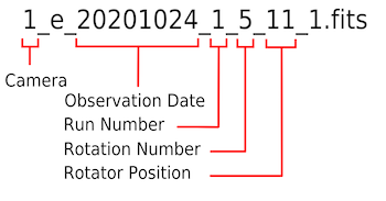
Example MOPTOP filename which is defined below.
Image © 2020 Doug Arnold
The first few terms (separated by underscores) are the usual:
- instrument label (cameras "1" and "2" in MOPTOP's case)
- observation type ("e" for science exposure, "s" for standard, "f" for flat)
- observation date = date of start of night (YYYYMMDD); does not change after midnight
- run number = the "run" or observation number for that instrument for the night
The next two terms are unique to MOPTOP:
- rotation number = the number of the current waveplate rotation
- rotator position = the current angular position of the waveplate, ranging from 1–16
The last term is as normal:
- flag that shows the reduction status of the file (0 = raw, 1 = reduced)
Data Reduction Pipeline
MOPTOP raw frames undergo bias subtraction, dark subtraction and flat fielding to remove the normal instrumental detector signatures. The pipeline is automated and runs on all data before they are stored in the archive and distributed to users.
Bias and Dark
Since there are only two possible exposure times to consider (fast and slow rotor), no scaling is needed to account for varying integration times and there is no need to separate bias from dark contributions to the signal. Bias and dark signal are independent of rotor position. The pipeline maintains and subtracts a combined ‘bias-plus-dark’ frame form every image.
Flat-field
(Caution with moptop photometry)
Each frame is divided by a flat-field image. The flat field being applied is an average stack of all sixteen rotor positions. That is, the same flat field is used for all sixteen frames in a rotation set. A separate flat field image is created for each filter. This means it well represents flat field effects deriving from the pixel-to-pixel sensitivity variations of the detector, wavelength dependence of the filters and instrumental vignetting of beam. It will not represent and correct any polarisation dependent features of the illumination pattern.
Instrument performance analysis is still ongoing but we currently believe this bias is corrected when using the differential analysis of the signal from the two cameras which is described in the "Deriving Polarisation" section below. However, we currently urge caution about using single-camera MOPTOP data for photometry. It is anticipated the flat field might introduce systematic errors for photometry, but not polarimetry.
WCS
A World Coordinate System (WCS) is applied to every image:
- All frames from a specific observation are co-added to create a high signal-to-noise image stack of the entire integration
- Sources are detected in that image using SExtractor
- A WCS is created using imwcs software, based on cross matching to the USNOB-1 or 2MASS Point Source catalogues
- The WCS is then transcribed into each individual frame and the stack discarded
In cases where the WCS fit fails, an approximate WCS is constructed on the basis of the telescope's blind pointing.
Deriving Polarisation
(Most of the information in this section is adapted from "Characterisation of a dual-beam, dual-camera optical imaging polarimeter", Shrestha et al, Monthly Notices of the Royal Astronomical Society, Vol 494, Issue 4, 2020. The paper is referred to as "Shrestha (2020)" in this text)
If time resolution during the observation is not important, all frames with the same rotator position can be stacked to obtain 16 frames per camera, each stacked frame corresponding to a 22.5° rotation of the waveplate.
Reduction begins by first using aperture photometry to extract sky-corrected source counts. Two means of converting this data to polarisation values are outlined in Shrestha (2020), namely the one and two-camera techniques. The two-camera technique however produces better results than the one-camera technique; it provides less error in degree of polarisation, and less scatter in Stokes q & u.
For this reason, the example that follows is of the two-camera technique. For brevity also, we show only half of what we can calculate from the 16 waveplate positions — remember that we can get four Stokes q and u values when applied to all 16 waveplate positions.
Obtaining polarisation of a source from the post-pipeline reduced data is achieved by:
- Correcting for the sensitivity difference between camera 1 and camera 2 by calculating the sensitivity factor
- Applying this sensitivity factor to correct the counts from camera 2
- Calculating the Stokes parameters q and u from the variation in counts with waveplate angle position
- Accounting for instrument polarisation
- Calculating percentage polarisation and position angle
Each of these steps are described in turn below.
1. Calculate sensitivity factor between cameras
First we must make sure the the two MOPTOP cameras have the same effective sensitivity. Let m and n be the observed counts from camera 1 and camera 2 respectively. Taking positions 1 and 3, equation 16 in Shrestha (2020) gives the relative sensitivity factor F as:
\[ F = \sqrt{\frac{n_{1}\,n_{3}}{m_{1}\,m_{3}}} \]
For example, to calculate this factor for Stokes parameters u and q for rotor positions 1 and 2:
\[ F_{1q} = \sqrt{\frac{n_{1}\,n_{3}}{m_{1}\,m_{3}}} \] \[ F_{2q} = \sqrt{\frac{n_{5}\,n_{7}}{m_{5}\,m_{7}}} \] \[ F_{1u} = \sqrt{\frac{n_{2}\,n_{4}}{m_{2}\,m_{4}}} \] \[ F_{2u} = \sqrt{\frac{n_{6}\,n_{8}}{m_{6}\,m_{8}}} \]
2. Correct camera 2 counts
With these sensitivity factors we can correct the counts for camera 2 to end up with corrected counts c and d for all positions for camera 1 and camera 2 respectively:
\( c_{1} = m_{1}, \quad d_{1} = n_{1} / F_{1q} \)
\( c_{2} = m_{2}, \quad d_{2} = n_{2} / F_{1u} \)
\( c_{3} = m_{3}, \quad d_{3} = n_{3} / F_{1q} \)
\( c_{4} = m_{4}, \quad d_{4} = n_{4} / F_{1u} \)
\( c_{5} = m_{5}, \quad d_{5} = n_{5} / F_{2q} \)
\( c_{6} = m_{6}, \quad d_{6} = n_{6} / F_{2u} \)
\( c_{7} = m_{7}, \quad d_{7} = n_{7} / F_{2q} \)
\( c_{8} = m_{8}, \quad d_{8} = n_{8} / F_{2u} \)
3. Calculate Stokes q and u
Corrected counts can now be used to calculate Stokes Q, U and I:
\( Q_{1} = c_{1} - d_{1} \)
\( U_{1} = c_{2} - d_{2} \)
\( I_{1} = \left( c_{1} + d_{1} + c_{2} + d_{2} \right) / 2 \)
\( q_{1} = Q_{1} / I_{1} \)
\( u_{1} = U_{1} / I_{1} \)
\( Q_{2} = -(c_{3} - d_{3}) \)
\( U_{2} = -(c_{4} - d_{4}) \)
\( I_{2} = \left( c_{3} + d_{3} + c_{4} + d_{4} \right) / 2 \)
\( q_{2} = Q_{2} / I_{2} \)
\( u_{2} = U_{2} / I_{2} \)
The final q,u are then the averages of the two values. In this way a single rotation in the instrument consists of 32 images (16 from each camera) and yields four independent, time-resolved q,u pairs.
\(q = (q_1 + q_2)/2 \)
\(u = (u_1 + u_2)/2 \)
calculating the error in Stokes q and u
The error in Stokes q and u are found by propagating the errors in the counts from the photometry. Let merr and nerr be the error in counts from cameras 1 and 2 respectively, and let qerr and uerr be the errors in q and u respectively.
If we then set:
\[ A_{q} = { \left\{ n_{err_{1}}^2 + \left(\frac{m_{3}}{2\,n_{1}\,n_{3}\,m_{1}}\right)^2 \left(\frac{1}{n_{1}\,n_{3}\,m_{1}}\right)^2 \left[ \left(\frac{n_{err_{1}}}{n_{1}}\right)^2 + \left(\frac{n_{err_{3}}}{n_{3}}\right)^2 + \left(\frac{m_{err_{1}}}{m_{1}}\right)^2 \right] + \left(\frac{m_{err_{3}}}{m_{3}}\right)^2 \right\} }^{\frac{1}{2}} \]
and
\[ A_{u} = { \left\{ n_{err_{2}}^2 + \left(\frac{m_{4}}{2\,n_{2}\,n_{4}\,m_{2}}\right)^2 \left(\frac{1}{n_{2}\,n_{4}\,m_{2}}\right)^2 \left[ \left(\frac{n_{err_{2}}}{n_{2}}\right)^2 + \left(\frac{n_{err_{4}}}{n_{4}}\right)^2 + \left(\frac{m_{err_{2}}}{m_{2}}\right)^2 \right] + \left(\frac{m_{err_{4}}}{m_{4}}\right)^2 \right\} }^{\frac{1}{2}} \]
Then qerr and uerr are given by:
\[ q_{err} = q \cdot \left[ \left( \frac{A_{q}}{m_1F_{1q}-n_{1}} \right)^2 + \left( \frac{A_{q}}{m_1F_{1q}+n_{1}} \right)^2 \right] \]
\[ u_{err} = u \cdot \left[ \left( \frac{A_{u}}{m_2F_{1u}-n_{2}} \right)^2 + \left( \frac{A_{u}}{m_2F_{1u}+n_{2}} \right)^2 \right] \]
[Binder implementation of a Jupyter notebook of the above steps in full detail]
4. Account for instrument polarisation zero point
To continue, finding the true polarisation of the science target involves accounting for instrument polarisation too. This is done by also observing an unpolarised standard star:
If qt, ut are the stokes parameters of the target, and q0, u0 are the Stokes parameters of the unpolarised standard, then the corrected Stokes values of the target qc, uc, are:
\[q_{c} = q_{t} - q_{0}\] \[u_{c} = u_{t} - u_{0}\]
All calibration data to date show this instrumental q,u zero point to be stable with no detected drift over time. Only movement of the optics during hardware changes causes any jump in parameter values.
The dates of these hardware changes are listed at the top of this page, but are reiterated here for clarity —
- 2020-10-01 — Instrument commissioning begins, using two Andor Zyla cameras
- 2021-03-09 — Andor camera 1 replaced with same model after previous camera 1 fault
- 2021-09-20 — Switch to imaging only with Andor camera 1, after fault with Andor camera 2
- 2022-03-20 — Both Andor cameras replaced with PCO cameras, imaging with two cameras again
- 2024-09-13 — Primary mirror realuminised
Only a small number of people (mainly LT group internal) used MOPTOP during the early part of characterisation, so we are publishing just the parameters from the time of PCO camera deployment onwards (2022 March – present).
| filter | Stokes parameter |
Hardware Epoch | |
|---|---|---|---|
| PCO cameras in use 2022-03-20 to 2024-08-22 |
Post-realuminisation 2024-09-13 to present |
||
| B | q0 | 0.00127 ± 0.00016 | 0.0016 ± 0.0005 |
| u0 | -0.01219 ± 0.00019 | -0.0131 ± 0.0006 | |
| V | q0 | 0.00601 ± 0.00015 | 0.0067 ± 0.0003 |
| u0 | -0.02326 ± 0.00013 | -0.0248 ± 0.0005 | |
| R | q0 | 0.01163 ± 0.00017 | 0.0109 ± 0.0005 |
| u0 | -0.03140 ± 0.00019 | -0.0319 ± 0.0003 | |
| I | q0 | 0.01135 ± 0.00015 | 0.0112 ± 0.0002 |
| u0 | -0.03401 ± 0.00012 | -0.0344 ± 0.0003 | |
| L | q0 | 0.00787 ± 0.00018 | 0.0084 ± 0.0008 |
| u0 | -0.01979 ± 0.00028 | -0.0203 ± 0.0005 | |
We strongly encourage observers to process a couple of unpolarised stars from the MOPStand proposal (Recent Data or Data Archive) from around the date of their science observations. This quickly confirms that the instrument is stable and that your data really are consistent with the facility values we publish here. It also serves as a check for consistency of the sign convention between our published values and your own software. Our published values will be updated as and when they become available.
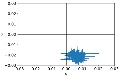
The instrumental q & u zeropoint values given above are derived from a large sample of repeated observations of unpolarised reference stars. The plot at right illustrates how the zeropoint values are grouped tightly at a fixed point in the q,u plane.
5. Percentage polarisation & position angle
Percentage polarisation
From qc and uc, percentage polarisation %p and position angle PA are given by:
\[ \%p = 100 \sqrt{{q_{c}}^2 + {u_{c}}^2} \] \[ PA = 0.5\;{\rm atan2}(u_{c},q_{c}) \]

A linear fit to the MOPTOP instrumental measurements and reference values for stars over a wide range of polarisation. MOPTOP R filter.
Ptrue = Pinst / 0.865
The polarisation figure must be corrected for instrumental depolarisation. This is simply a constant multiplicative correction that accounts for the polarisation efficiency of the instrument. It is derived by observing calibration standards and comparing the instrumental measurements to true values. All calibration data to date show this instrumental depolarisation to be stable with no detected drift over time. Observers can therefore use the following values derived during commissioning.
| date of observation | B | V | R | I | L |
|---|---|---|---|---|---|
| 2020-10-01 — 2022-03-19 | 0.79 | 0.83 | 0.86 | 0.76 | 0.88 |
| 2022-03-20 — present | 0.86 | 0.87 | 0.91 | 0.81 | 0.92 |
We strongly encourage observers to process a couple of highly polarised stars from the MOPStand proposal (Recent Data or Data Archive) from around the date of their science observations. This quickly confirms that your data really are consistent with the facility values we publish here and also serves as a check for consistency of the sign convention between our published values and your own software. These values will be updated as they become available.
Position Angle
The PA angle measured is relative to the position of the telescope and instrument. The position of the telescope is quantified using the ROTSKYPA fits header which gives the angle of rotation East of North on the sky. Corrected position angle is given by:
\[ EV PA = PA + ROTSKYPA + K \]
where K is correction angle that you calculate using the standards observed. Latest K-values for the pco.edge cameras installed in March 2022 are given below:
| date of observation | B | V | R | I | L |
|---|---|---|---|---|---|
| 2022-03-20 — present | 124.67 ± 0.47 | 122.80 ± 0.25 | 124.11 ± 0.19 | 124.08 ± 0.17 | 126.89 ± 0.34 |