

RINGO3
RINGO3 experienced a major hardware fault on 14th January 2020. With RINGO3's successor MOPTOP coming online soon, the decision was made to focus effort on that instrument rather than spend time repairing RINGO3. RINGO3 is therefore effectively decommissioned as of the above date, to be replaced with MOPTOP soon.
- Introduction
- Wavelength Ranges
- CCD Cameras
- Optical Performance
- Sensitivity
- Minimum Integration Time
- Saturation
- Data Reduction Pipeline
- Deriving Polarisation
- Phase 1 Guidelines
- Phase 2 User Interface Instructions
Introduction
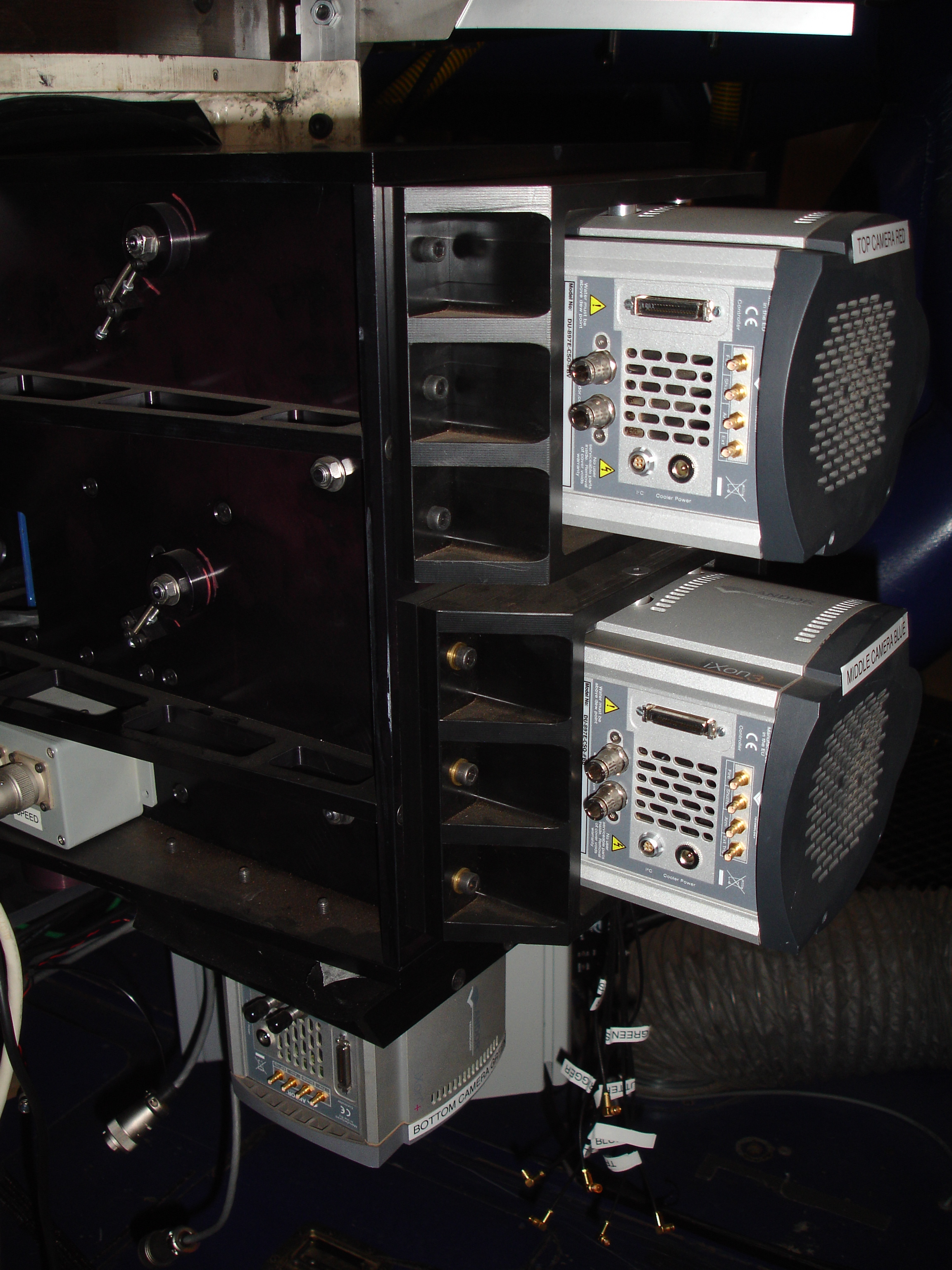
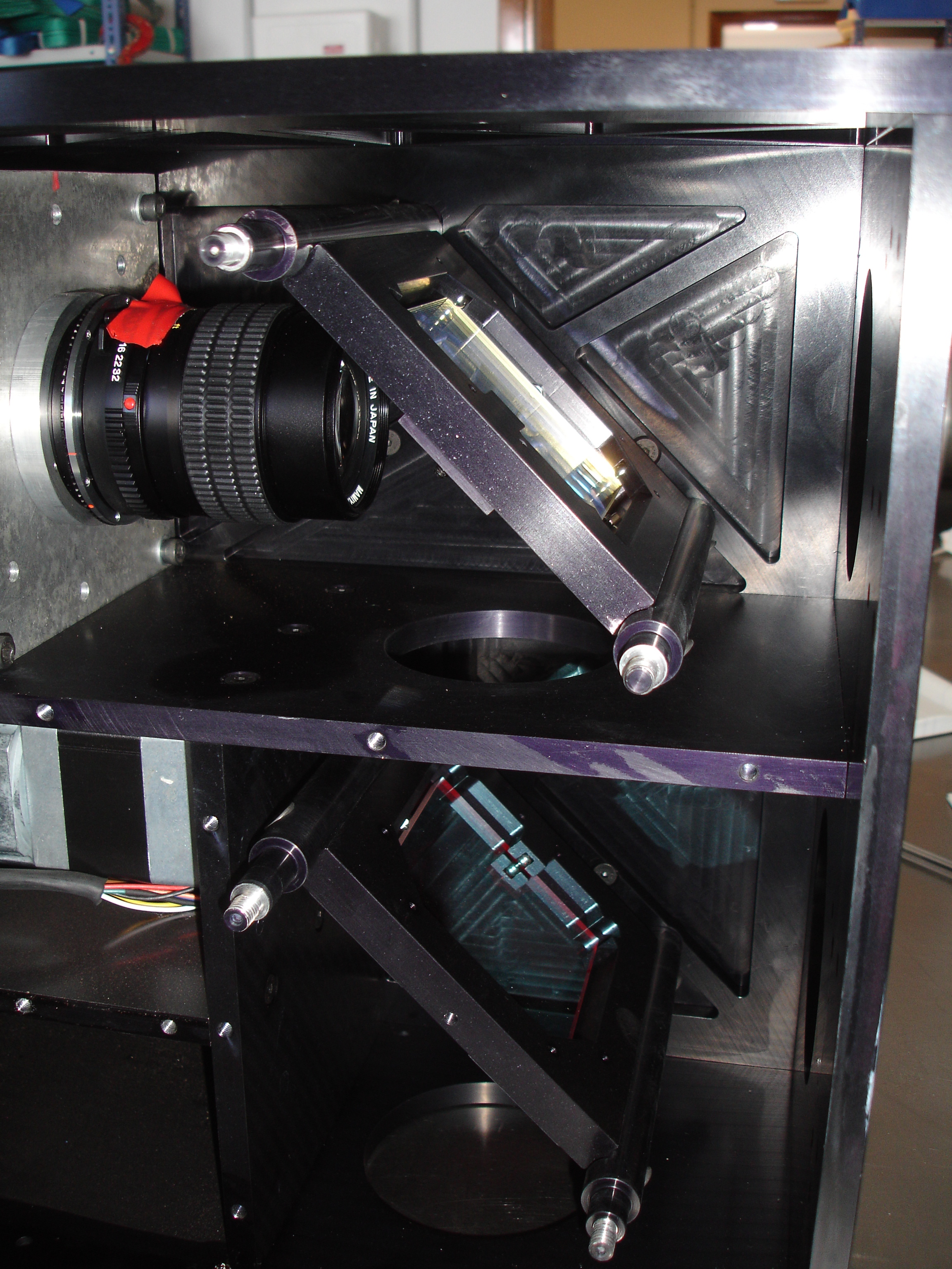
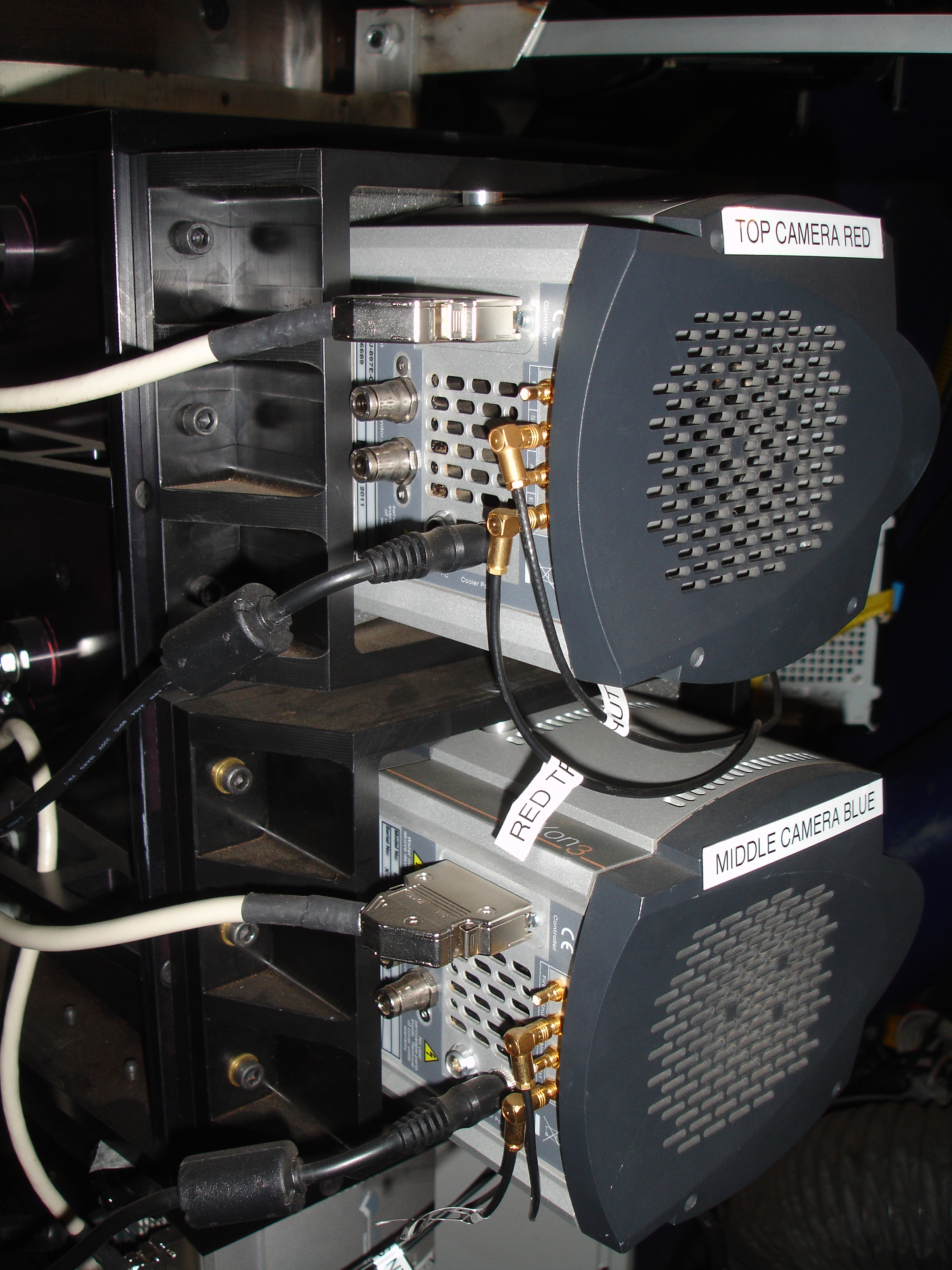
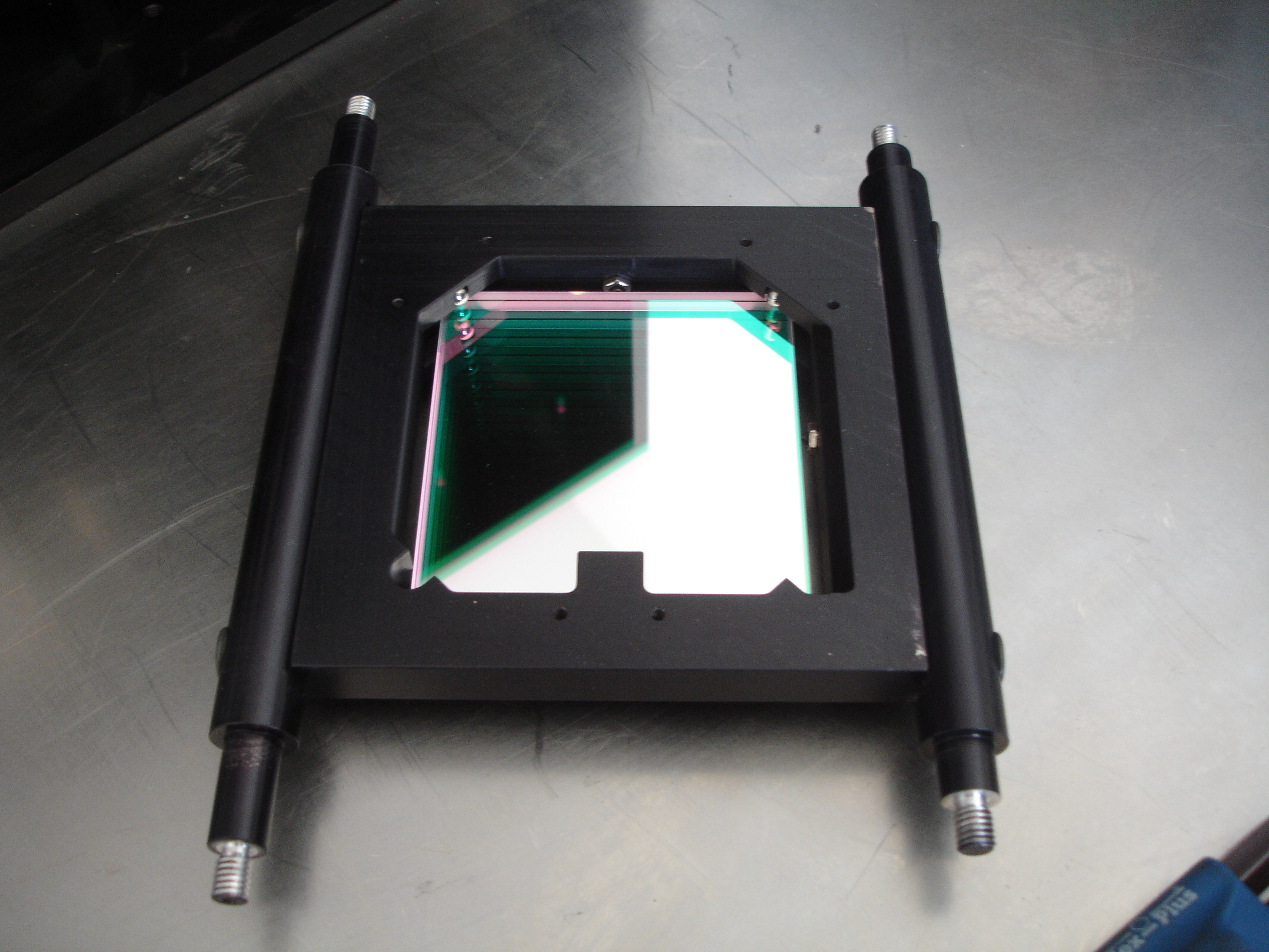
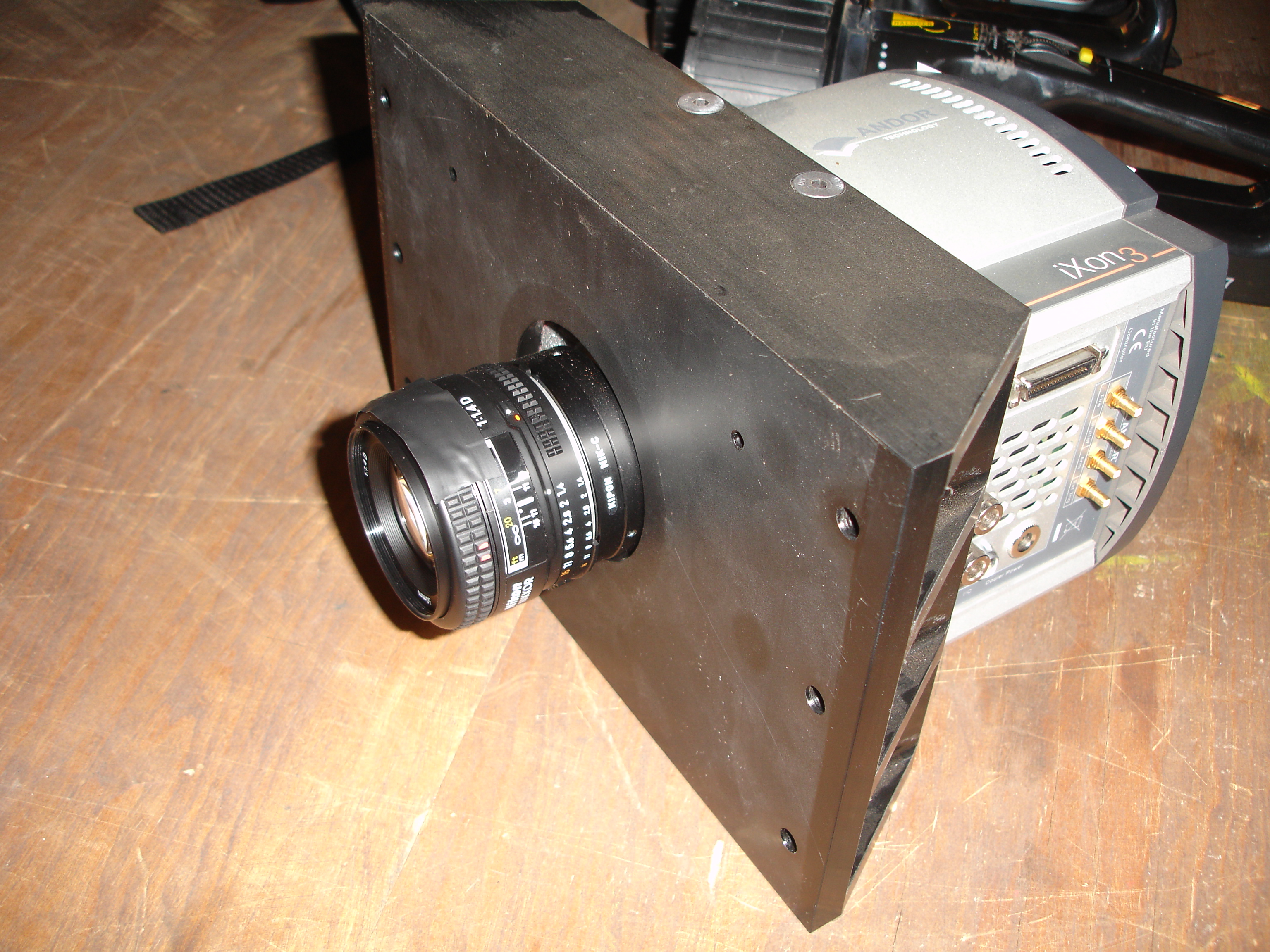
RINGO3 (shown here uncabled) is a fast-readout optical imaging polarimeter. It uses a polaroid that rotates every ~2.5s to measure the polarisation of light entering the instrument. A pair of dichroic mirrors split the light into three beams for simultaneous polarised imaging in three wavebands using three separate Andor cameras (two of which are shown here).
Exposures are synchronised with the phase of the polaroid's rotation and each camera receives eight exposures per rotation. All images for each octal phase are stacked to obtain the final signal at each phase in the polaroid's rotation. Observing for longer and thus stacking more images in each octal phase increases the signal-to-noise ratio obtained and therefore improves the polarisation accuracy of the observation.
RINGO3 was commissioned in early 2013. However, observations later in the year demonstrated a problem with polarisation induced by the two dichroic mirrors. This instrumental polarisation unfortunately changes with the mount angle (the angle of the cassegrain stage) used for the observations. The problem is described in more detail here. All users of RINGO3 in 2013 are encouraged to read this document and/or contact us (the LT support astronomer) to discuss their observations PRIOR to publishing.
To combat this problem, in December 2013 we inserted a depolarising Lyot prism into the beam, after the rotating polaroid but before the beam reaches the first dichroic mirror. Note that downstream of the rotating polaroid all one needs to measure is the intensity of the light, not its polarisation state. Prospective users of RINGO3 are encouraged to read this document for further details. We are now confident in the calibration of RINGO3, and there is no need to do observations at multiple mount angles as we were recommending in 2014.
From installation until June 2015 the rotor turned at roughly 1Hz. From 29th June 2015 onwards the rotor is running at ∼0.4Hz. Procedures for data handling, processing and analysis are unaffected by this change. Total dwell time on a target is unchanged so no change is required to phase2 configurations, but it means the integration time per frame is now about 0.32sec instead of 0.125sec. Targets that were close to saturating at 1Hz may now be saturated.
Wavelength Ranges
RINGO3 uses three cameras, called "Red", "Green" and "Blue", with approximate wavelength ranges of:
- Red: 770-1000 nm (FITS file prefix "d")
- Green: 650-760 nm (FITS file prefix "f")
- Blue: 350-640 nm (FITS file prefix "e")
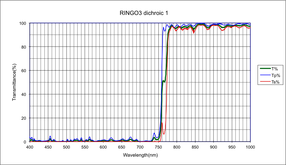
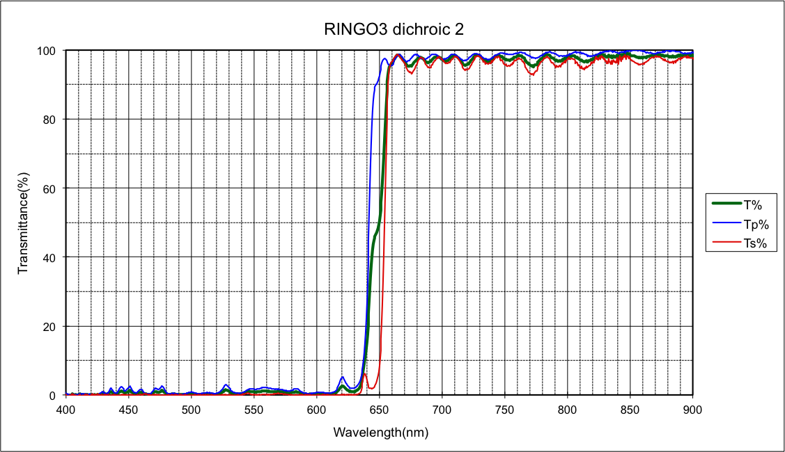
The wavelength ranges are dictated by the dichroics in the optical layout which split the beam between the three cameras. Their transmission graphs are below (click each graph for a bigger version):
|
|
The dichroics have been specially designed to have a minimal change of wavelength depending on polarisation angle. Nevertheless there is still a small (10nm) discrepancy between the orthogonal s and p polarisation states that should be taken into account in your data analysis if the source has very extreme colours, or strong line emission/absorption in the crossover regions.
CCD Cameras
Each camera uses a 512x512 pixel EMCCD and has negligible dark current. The EMCCD gain can be set to values of 5, 20 or 100. Unless the source is very bright, we recommend EMGAIN=100, which will correspond to a gain value of around 0.32 electons/ADU in a single frame. Since the data pipeline automatically stacks images to create a mean frame from a given polaroid ROTOR position, the final gain of your images can be calculated by multiplying 0.32 by the number of frames that have gone into making the stack (FITS keyword NUMFRMS). For example, if the stack contains 10 images, the effective gain for that image would be 3.2 electrons/ADU.
The effective gain of a stacked image is noted in the FITS keyword GAIN (not to be confused with the EMGAIN header).
Optical Performance
A different camera lens is used on the red arm of the instrument as opposed to the blue and green arms, giving slightly different plate scales and vignetting of the beam. The following parameters have been derived on sky:
| Before 2014-06-08 | Before 2014-06-08 (8th June 2014) | ||||||||||||||||
|---|---|---|---|---|---|---|---|---|---|---|---|---|---|---|---|---|---|
|
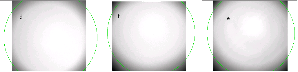 Typical RINGO3 flats linearly scaled (0-1). Green circle defines radius of 50% throughput. Click for bigger version. | ||||||||||||||||
| After 2014-06-07 | After 2014-06-07 (7th June 2014) | ||||||||||||||||
|
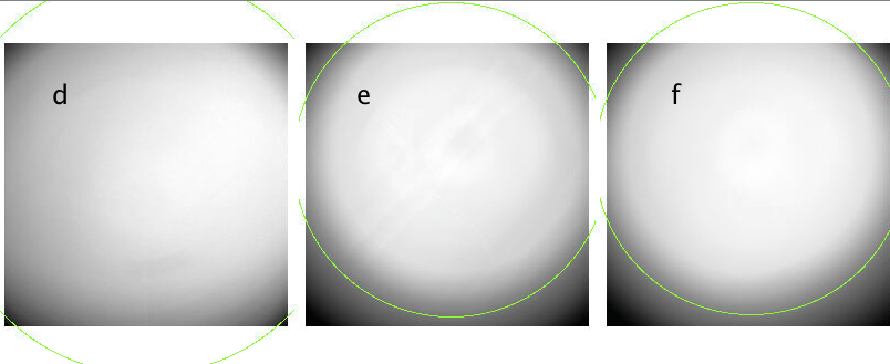 Typical RINGO3 flats linearly scaled (0-1). Green circle defines radius of 50% throughput. Field on camera d is substantially increased and almost entire frame is above 50%. Cameras e and f are largely unchanged. Click for bigger version. | ||||||||||||||||
Test observations on a highly-polarised twilight sky indicate that the variance across the unvignetted field is about 2% on a polarisation measurement of approximately 75%. The field variance is expected to scale with the polarisation of the source. We therefore expect to see less than 1% variance on polarisation measurments of astronomical sources with polarisations up to about 30%, regardless of where the target lands in the ~4 arcmin unvignetted field. This variance is expected to be smaller than the photometric errors associated with sources that are fainter than 13th or 14th magnitude.
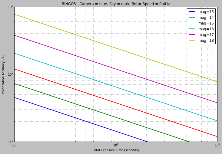
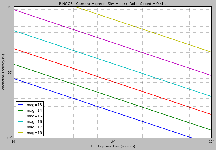
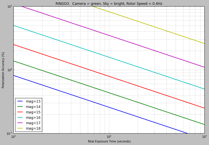
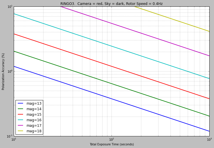
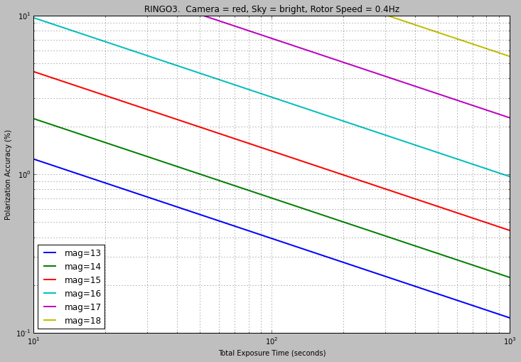
Sensitivity
Updated 1st Oct 2015
In imaging polarimetry, the polarisation accuracy (ΔP) is related to the signal-to-noise ratio (SNR) by:
-
SNR = 1.414 / ΔP
For example, to obtain a polarisation accuracy of 1.0% a SNR of approximately 141 is theoretically required.
If the noise associated with each integrated flux measurement is predominantly shot noise from the source itself (i.e. ignoring the sky background, readnoise and dark current), then the SNR can be estimated from the instrumental zero-point (ZP) for each camera. ZPs for RINGO3's three cameras are presented in the table below.
| Camera | Red 'd' | Green 'f' | Blue 'e' |
|---|---|---|---|
| Corresponding optical filter band | I | R | V |
| Zero-Point (mag)* | 21.0 | 21.8 | 23.0 |
*equivalent to 1 photon per second
The above ZP values may be used to directly estimate the integrated flux (again, the sum of values from eight stacks, divided by 2.0 - in photons per second) that will be detected in a second for a given source B,R or I-band magnitude. This SNR can then be used to estimate polarisation accuracy for a 1 second observation (the SNR may be increased in the usual way by obtaining longer observations).
Example:
-
Target R = 16.0 mag
ZP of the Green ("R-band") camera = 21.8
Equivalent flux from target = 200 photons/second
-
In 1 second, SNR = 14, so ΔP ~ 10%
In 100 seconds, SNR = 140, so ΔP ~ 1.0%
Note that the instrumental polarisation induced by the dichroics (described in the introduction at the top of this page) means that a polarisation accuracy of better than 0.3% is probably not possible, regardless of the SNR achieved.
RINGO3 is now also included in the Imaging Exposure Time Calculator. although the graphs below are probably more accurate.

Minimum Integration Time
The overheads in initialising the instrument for an exposure mean that exposures shorter than about 5 - 6 sec are likely to be incomplete and unusable. We therefore recommend a minimum integration time of 20 sec for all RINGO3 exposures. Compared to slew and other overheads, the difference between 5 sec and 20 sec integration will not be a significant impact on total time used. Remember that due to the way Ringo3 operates, averaging multiple short, fixed length exposures to build up the requested integration, a longer integration does not lead to greater risk of saturation. It only creates higher signal-to-noise in a frame with the same mean signal.
Saturation
IMPORTANT: to avoid saturation, which may permanently degrade the response of the EMCCD, great caution must be exercised with any field containing objects brighter than 10th magnitude. Similar to the note above, shorter integrations do not reduce the risk of saturation. The 10th magnitude limit is set to prevent saturation in a single 1/3rd second exposure at EMGAIN=100.
If you have a target (or near by companion object in the field) brighter than 10th magnitude it is still possible to use RINGO3 but you must turn down the EMGAIN configuration in your phase2 sequence from the default value of 100. For example, the 8th and 9th magnitude calibration standards are observed with EMGAIN=20.
If any of this is unclear, rather than risk the instrument, please contact us in advance regarding any bright targets.
Standards
Zero-polarised and polarised standards are observed for RINGO3, selected from the same list as used by RINGO2, every night. Users do not need to request poliarmetric standards in their Phase 1 proposal, nor schedule them in their Phase 2 submission.
Two types of standard are necessary to reduce RINGO3 data; unpolarised stars, and objects with known polarisation. The unpolarised standards are necessary to remove the instrumental polarisation from the data. The polarised standards allow you to calibrate the effect of instrumental depolarisation.
These standards are used to remove the instrumental signature in the polarimetry measurements, they are not primarily intended for photometric calibration and are not effected by issues such as airmass. This, and the fact that instrumental components are stable on timescales of many months, mean there is no need to observe the same standard multiple times through the night. Our tests have demonstrated that better calibration is obtained by using a variety of different reference stars observed over a few nights either side of the science observation rather than a single standard observed multiple times on the night of the science frame. Our automated standard scheduling takes this into account and follows a different strategy than, for example, the photmetric standards on IO:O. We are in the process of developing a calibration procedure document, but in the mean time interested observers who need assistance should contact us to discuss Ringo3 calibrations.
In general we recommend using a MOUNT position angle of zero for all RINGO3 observations. Calculation of a true sky position angle for your data (and hence polarisation angle) is possible by using FITS keywords. In the FITS headers the sky position angle is stored in ROTSKYPA and the mechanical mount position in ROTANGLE.
Because these standards are used for polarimetric calibration and not photometric calibration there are no particular actions required, but be aware that the very bright and fainter stadards are observed using a different camera gain settings to prevent saturation.
Standards currently being observed with RINGO3 are taken from:
-
Schmidt, Elston and Lupie 1992,
The HST Northern Hemisphere Grid of Stellar Polarimetric Standards,
AJ, 104, 1563.
Hough et al. 2007, Low Polarisation Standards, ASP Conf. Ser. 364, 523.
Data Reduction Pipeline
Each camera (d, e and f) produces a separate set of FITS files. The software pipelines largely treat the instrument as three independent cameras each with their own calibrations. Currently all three cameras use exactly the same algorithms and configuration options.
As RINGO3 produces approximately 24 CCD frames every 2.3 seconds (one per camera, per polaroid rotor position, running at approximately 0.4Hz), it is not practical to archive or distribute the raw data from the instrument. The data reduction pipeline at the telescope therefore stacks all of the frames at a given rotor position within a multrun and normalises by the number of frames in the stack. A multrun of any length will therefore produce 24 files, named [d,e,f]_*_N_0.fits where N varies from 1 to 8. These mean-stacked frames are then transferred back to the data archive at LJMU for normal CCD reductions. Note that this means a one minute or a ten minute integration will yield a FITS file with the same mean counts level. The longer integration will have a higher signal-to-noise ratio and a different effective gain which is calculated and written into the FITS header.
The primary data product is an averaged stack of the entire integration time, however for long integrations the FITS files contain multiple image extensions with the data broken down into a sequence of 1 minute blocks to allow time resolved studies. If you need a time series broken down more finely than 1 co-added frame per minute, please contact us to discuss the requirements.
The basic CCD reduction pipeline (darks, flats etc) is identical to that used on all the LT imaging cameras, but the need to collate and pre-stack the raw data adds several extra pre-processing steps which are unique to RINGO3.
-
On-site Pre-Process Performed at Telescope
- Runs at dawn after enclosure closes.
- Ignore any integrations too short to generate less then 2 full rotations of the rotor. Exposures that are too short will not be processed. See "Minimum Integration Time" above.
- Group integration into 1 minute blocks. Each block (except the last) consists of an integer number of rotor turns so the duration will typically be between 59 and 61 seconds but eacvh rotor position in a single block always contains the same number of frames. The final block contains whatever is left, may be substantially less then 60sec and the 8 rotor positions may contain different numbers of combined frames. FITS headers are populated with appropriate values to show how many frames were used in each stack.
- Simple average stacks are made without any rejection of deviant pixel values for each of the one minute blocks and for the entire integration time.
- Header keywords are generated independently to give the start, end, duration, effective gain, number of rotor turns and number of frames combined for each of the one minute blocks.
- Average rotor speed for the entire integration is derived from start and end times and number of rotor turns in the entire integration. This average is applied to FITS headers for all the 1 minute blocks. Intra-night stability of rotor speed is 0.01sec per rotation.
- For each one minute block, the image background level is estimated as the average counts in the top two corners of the image. Since the effective integration time in all these images is only ∼1/3rd second (1/8th sec prior to July 2015), this background level is dominated by the CCD bias level and will later be used in conjunction with actual dark frames in order to estimate the CCD bias, not the sky flux.
- Camera f is reflected so that all three cameras show the same orientation to the sky.
- The one minute blocks are assembled into FITS image extensions behind the primary FITS image which contains the full integration stack.
- These multi-extension, stacked, raw frames are transferred to Liverpool for the normal CCD reductions.
-
Bias Subtraction
The camera bias levels are found to vary ±1ADU on time scales of a few days but there are no overscan strips from which to directly measure the instantaneous value. To track these changes a single fixed bias level is derived for each camera for each night. All the images for the night are inspected and the 5% with the darkest background levels are selected. This rejects any twilight or moonlit images. Since effective integration times are fixed as 1/8 of the rotor speed, the sky flux in the vignetted field corners is essentially zero and this provides an adequate bias estimate. The bias level for the night is set to be the average from the darkest 5% of images. Dark frames are also obtained daily and if these yield a lower bias estimate, that value is used instead in order to allow for the case where maybe every night-time exposure was Moon affected.
-
Dark Subtraction
Dark frames are collected automatically every evening as an average stack of 1000 dark frames each with the same 1/8-rotation per-frame integration time as the science data. Since the effective integration time is fixed on all frames there is no need to separate spatial structures in the bias from those in the dark and both are subtracted together in single operation.
-
Flat Fielding
Twilight flats are manually obtained as required and stored in a library in the data archive. All images are divided by the flat field which has been normalised to unity near the frame centre.
-
Bad Pixel Mask
No cosmic ray rejection or bad pixel mask is applied since it is important for users performing accurate photometry to know exactly what masking has been applied. For integrations longer than one minute, the individual substacks in the FITS extensions provides a clear check of any suspected cosmic rays and bad pixels.
-
Fringe Frames
No fringing has been detected or automatically corrected.
-
Sky Subtraction
No sky subtraction is performed. The sky background in the distributed images is near zero because each image is the average of many short exposures. A one minute or ten minute integration will have the same background level (near zero) but different signal-to-noise and effective gain.
Deriving Polarisation
Two types of standard star observations (zero-polarization and polarized) are necessary to reduce RINGO3 data, which should have been obtained with the same mechanical mount position angle as the science data. The mount angle is specified in the FITS header by keyword ROTANGLE.
- Carry out sky-subtracted photometry on the frames corresponding to your zero polarized standard(s). You will have eight measurements (one per rotor position) per target.
- Carry out sky-subtracted photometry on the frames corresponding to your polarized standard(s) and science target(s)
- For each rotor position, divide the counts from the polarized standards and science targets by those from your zero-polarized standard. This process (analogous to flat-fielding) removes the effect of the instrumentatal polarization from your data.
- For each polarized standard and science target use the
equations outlined in Clarke &
Neumayer 2002 to calculate q and u, and hence the degree of
polarization [ P = q2 + u2 ] and
position angle [ PA = 0.5 arctan(u/q) ] relative to the mount.
Note that rotor positions correspond to the nomenclature used in
Clarke & Neumayer according to the scheme:
ROTOR POSITION Clarke & Neumayer
nomenclature1 A1 2 B1 3 C1 4 D1 5 A2 6 B2 7 C2 8 D2 - Plot a graph of the observed vs actual values for the polarized standards. Place your measured value for your science target on the graph to calculate its true polarization.
IMPORTANT : Dates of hardware changes
Because the relative physical alignment between the polarizer, the rotor and the CCD array is critical to the data reduction it is important to use only the correctly matched flat fields and standard stars to analyse science data. You cannot use standards before and after any hardware reconfiguration interchangeably. The following list gives dates on which hardware were changed. The individual details of the change are not so important; just make sure your standards and science frames are not separated by any of these dates.
- 2013-01-23 Field lens removed and polarizer moved.
- 2013-12-12 Depolariser installed between the rotating polaroid and the first dichroic mirror.
- 2014-06-08 Field lens changed. Depolariser moved to collimated beam.
- 2015-06-29 Mirror recoating gives large throughput increase. Rotor slowed from 1Hz to 0.4Hz. Due to other hardware alignment changes, the numerical sign of Stokes parameters flipped. Amplitudes remain roughly consistent but comparing before/after this date; q will be approximately the same and u inverts its sign ±.
- 2018-06-27 Tertiary feed mirror cleaning gives throughput increase.
Please feel free to contact the LT Support Astronomer to discuss the impact any of these changes might have had on your data.
Phase 1 Guidelines
For RINGO3 a simple 60 second slew overhead is all that is required. No filter changes are possible, and the readout time is negligible.
Phase 2 User Interface Instructions
Guidelines on how to prepare observations are given in the Phase 2 web pages. Note in particular the instrument-specific User Interface Instructions. The phase 2 "Wizard" should always be used to prepare observations. Groups that can not be prepared with the wizard should be discussed with LT Phase 2 support. Note that LT staff do not routinely check observing groups, and that observing groups are active for observation as soon as they are submitted. Please do contact us if you have any questions about your observations.
Using the Phase 2 GUI to program the LT to use RINGO3 is essentially the same as for using RINGO2. Users should follow these instructions, obviously selecting RINGO3 in the instrument drop-down box instead of RINGO2.
Unless your target contains a target brighter than 10th magnitude we recommend that all users select a Gain of 100 when preparing their observations. Please contact phase2 support if you think a gain of 5 or 20 might be more appropriate for your target.
